Geometry and indexing

Coordinate system

Grids are described in polar coordinates \((x, r, \theta)\) where \(x\) is the axial direction, \(r\) the radial direction, and \(\theta\) the circumferential angle measured clockwise when looking upstream, giving a left-handed system opposite to the right-handed convention common in general CFD codes. A consequence is that cell volumes computed from the divergence theorem are positive when the index triple \((i, j, k)\) is a left-handed set, i.e.when \(i\), \(j\), and \(k\) increase in the \(x\), \(r\), and \(\theta\) directions respectively.

For the area and volume calculations the coordinates are first mapped to a pseudo-Cartesian space \((x, r, r\theta)\) which linearises the circumferential metric and allows standard vector identities to be applied. The implementations of all calculations below are in geometry.f90.

Face areas

Face area vectors are computed using Gauss’s theorem. Vertices are expressed in pseudo-Cartesian coordinates \((x, r, r\theta)\) and centred at the face centroid to reduce round-off. Let \(\mathbf{v}_e\) be the midpoint of edge \(e\) and \(\delta\mathbf{v}_e\) the vector between its endpoints. Each component \(d\) of the area vector is

\[\delta A_d = \tfrac{1}{2} \sum_{e=1}^{4} \mathbf{F}_d(\mathbf{v}_e) \cdot \delta\mathbf{n}_e\]

For each direction \(d\), the vector field \(\mathbf{F}_d\) is chosen with the \(d\)-th component set to zero and the remaining two components equal to the corresponding coordinates, so that \(\nabla \cdot \mathbf{F}_d = 2\). The edge normal \(\delta\mathbf{n}_e\) is the signed 2D edge normal in the plane perpendicular to \(d\), padded with zero in the \(d\)-th position. Together \(\mathbf{F}_d \cdot \delta\mathbf{n}_e\) reduces to a cross-product of the two in-plane edge components, and summing over the four edges via Gauss’s theorem yields the projected face area.

For a triangular face with vertices \(A, B, C\) the area vector is

\[\delta\!\mathbf{A} = \tfrac{1}{2}\, \overrightarrow{AC} \times \overrightarrow{AB}\]

Cell volumes

Cell volumes are obtained from the divergence theorem. Using the vector field \(\mathbf{F} = (x,\, r/2,\, r\theta)\), for which \(\nabla \cdot \mathbf{F} = 3\) in cylindrical coordinates, the volume of a cell is

\[\delta\mathcal{V} = \frac{1}{3} \oint \mathbf{F} \cdot \mathrm{d}\mathbf{A} = \frac{1}{3} \sum_{f=1}^{6} \mathbf{F}_f \cdot \delta\mathbf{A}_f\]

where \(\mathbf{F}_f\) is evaluated at the face centre, taken as the average of the four corner nodes of each face.

Minimum length scale

The minimum bounding length scale of a cell is

\[\delta l_\mathrm{min} = \frac{\delta\mathcal{V}} {\max(\|\delta A_i\|, \|\delta A_j\|, \|\delta A_k\|)}\]

where each face area magnitude is the larger of the two opposing faces to give a conservative (smallest) estimate.

Smoothing length scales

Anisotropic smoothing uses a per-direction length scale obtained by dividing the cell volume by the mean of the two opposing face area magnitudes,

\[\delta l_d = \frac{\delta\mathcal{V}} {\tfrac{1}{2}\left(\|\delta A_d^-\| + \|\delta A_d^+\|\right)}, \qquad d \in \{i, j, k\}.\]

The smoothing ratio in each direction is the ratio of the smallest directional length to that direction’s length,

\[\ell_d = \frac{\delta l_\mathrm{min}}{\delta l_d}, \qquad \delta l_\mathrm{min} = \min(\delta l_i, \delta l_j, \delta l_k),\]

so that \(\ell_d \le 1\) with equality in the direction of the smallest length scale. These cell-centred ratios are interpolated to nodes and rescaled so that the three components sum to three, recovering \(\ell_d = 1\) for an isotropic cell.

Indexing

For a block whose nodes have shape \((n_i, n_j, n_k)\), all arrays take one of three shapes depending on where the quantity is located.

Location	Shape	Description	Examples
Node	\((n_i,\; n_j,\; n_k)\)	Vertices at corners of cell control volumes	Coordinates Conserved variables
Cell	\((n_i-1,\; n_j-1,\; n_k-1)\)	Hexahedral cell \((i,j,k)\) is enclosed by nodes \(i, i{+}1\), \(j, j{+}1\), \(k, k{+}1\)	Volumes Residual CFL
\(i\)-face	\((n_i,\; n_j-1,\; n_k-1)\)	Constant-\(i\) boundaries of each cell	Face areas Fluxes
\(j\)-face	\((n_i-1,\; n_j,\; n_k-1)\)	Constant-\(j\) boundaries of each cell	Face areas Fluxes
\(k\)-face	\((n_i-1,\; n_j-1,\; n_k)\)	Constant-\(k\) boundaries of each cell	Face areas Fluxes

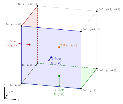
Multi-component quantities append a trailing dimension \(m\) so that the component index varies fastest, matching the column-major (contiguous last index) layout of the underlying Fortran arrays. For example, nodal velocity has shape \((n_i,\; n_j,\; n_k,\; 3)\) with the coordinate direction on the last axis, and cell CFL numbers have shape \((n_i-1,\; n_j-1,\; n_k-1,\; 5)\) with the equation index on the last axis.