Gas turbine Joule cycle

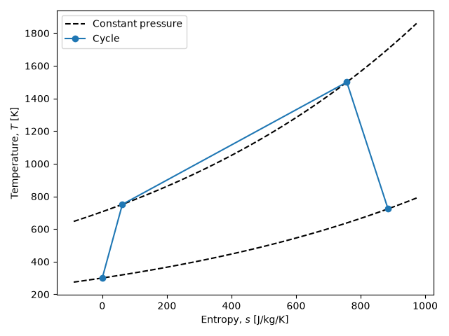
This example uses the ember.block.Block API to perform a thermodynamic analysis of a gas turbine operating on the Joule (Brayton) cycle with non-isentropic turbomachinery, then draws the corresponding temperature–entropy diagram.

Because all property evaluations go through a ember.fluid equation of state assigned with Block.set_fluid, the Block operations are working-fluid independent: only the object passed to Block.set_fluid would change.

import numpy as np
import matplotlib.pyplot as plt

import ember.block
import ember.fluid

Working fluid and cycle parameters

We model air as a perfect gas and specify the cycle by its overall pressure ratio, a (common) polytropic-style isentropic efficiency for both the compressor and turbine, and the ratio of turbine-inlet to compressor-inlet temperature.

fluid = ember.fluid.PerfectFluid(cp=1005.0, gamma=1.4, mu=1.8e-5, Pr=1.0)

PR = 20.0  # Overall pressure ratio
eta = 0.9  # Turbomachinery isentropic efficiency
Theta = 5.0  # Turbine-inlet to compressor-inlet temperature ratio, T3 / T1

Evaluating the cycle stations

A single Block with four entries holds the four cycle stations: compressor inlet (1), compressor exit (2), turbine inlet (3) and turbine exit (4). Each thermodynamic state is fixed by two properties, and the isentropic efficiencies relate the real enthalpy rise/drop to the ideal one.

block = ember.block.Block(shape=(4,)).set_fluid(fluid)

# (1) Compressor inlet, atmospheric conditions
P1 = 1e5
T1 = 300.0
block[0].set_P_T(P1, T1)

# (2s) Isentropic compressor exit: raised pressure, same entropy
P2 = PR * P1
block[1].set_P_s(P2, block[0].s)

# (2) Real compressor exit via isentropic efficiency
h1, h2s = block.h[:2]
h2 = h1 + (h2s - h1) / eta
block[1].set_P_h(P2, h2)

# (3) Turbine inlet at the specified temperature ratio
T3 = T1 * Theta
block[2].set_P_T(P2, T3)

# (4s) Isentropic turbine exit: dropped pressure, same entropy
block[3].set_P_s(P1, block[2].s)

# (4) Real turbine exit via isentropic efficiency
h3, h4s = block.h[2:]
h4 = h3 - (h3 - h4s) * eta
block[3].set_P_h(P1, h4)

<ember.block.Block object at 0x74ca693b5250>

Cycle efficiency

The thermal efficiency is the net specific work output divided by the heat added in the combustor.

h = block.h
wx_net = (h[2] - h[3]) - (h[1] - h[0])
q_in = h[2] - h[1]
eta_cycle = wx_net / q_in
print(f"Cycle thermal efficiency: {eta_cycle:.3f}")

Cycle thermal efficiency: 0.434

Temperature–entropy diagram

Finally we overlay the cycle path on the two constant-pressure lines that bound it. The constant-pressure lines are themselves evaluated with a Block, sweeping entropy at fixed pressure.

ni = 50
lines = ember.block.Block(shape=(2, ni)).set_fluid(fluid)
s_min, s_max = block.s.min(), block.s.max()
Ds = 0.1 * (s_max - s_min)
s = np.linspace(s_min - Ds, s_max + Ds, ni)
lines[0].set_P_s(P1, s)
lines[1].set_P_s(P2, s)
lines = lines.transpose()

fig, ax = plt.subplots()
const_P = ax.plot(lines.s, lines.T, "k--")
const_P[0].set_label("Constant pressure")  # Label only one of the two lines
ax.plot(block.s, block.T, "-o", label="Cycle")
ax.set_xlabel("Entropy, $s$ [J/kg/K]")
ax.set_ylabel("Temperature, $T$ [K]")
ax.legend()
fig.tight_layout()
plt.show()